THE CONSTRUCTION AND USE OF GRAPHS
The following table gives the average maximum temperature, to the nearest degree (in degrees Fahrenheit), at a certain town during the first six months of 1935:
| Month | Jan. | Feb. | Mar. | Apr. | May | June |
| Average maximum temperature | 44 | 48 | 52 | 56 | 64 | 72 |
It is usually easier to grasp the meaning of such a set of figures, if they are shown in the form of a picture, or graph. The figure shows them as a column graph.
The graph is drawn as follows:
1. Two lines called axes are taken, along which measurements may be made. The intersection of the axes is called the origin, and is usually denoted by the letter 0. It is usual to take lines at right angles as axes.
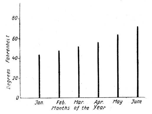
График температуры
2. The axes are labelled to show what quantites are measured along them.
3. The axes are graduated, in one case to show the various months, and in the other to show the temperature.
4. Along the first axis the months are represented at equal intervals.
5. Along the second axis the temperature is represented by a certain scale; in this case a small division is taken to represent 4°.
6. On the first axis, at each point which represents one of the months, a line is drawn parallel to the second axis; the length of this line represents the temperature.
7. The graph is given a title.
Note 1. It is usual to draw graphs on squared paper ruled in inches and tenths, or centimetres and millimetres. Such squared paper is not essential and, at a later stage, the pupil should be encouraged to draw rough sketches on ordinary paper.
Note 2. It is not essential to' show the zero mark on the axes. In the above table all the temperature lie between 44° and 72°, and there was no need to graduate the scale to show all the numbers from 0° to 80°. The alterations in temperature would have been as clearly shown, if along the second axis we had shown only the range from 40° to 80°. If we had done this, we could have taken a larger scale, say, a small division to represent 2°.
When the range of values to be shown is small, it is very important to choose a large scale. Consider a graph which shows that a man's temperature during a certain day moves between the limits 98.5° and 101.3° F.
Functions
If one variable changes when another variable is changed, we say that the first (or dependent variable) is a function of the second (or independent variable).
Thus, a boy's weight is a function of his age; the time of swing of a pendulum is a function of its length. In using the word function we do not imply the existence of an algebraic expression from which values of the function can be calculated; thus, although a boy's weight is a function of his age, there is no algebraic expression from which we can calculate his weight when we know his age. But when there is such a function, we call it an algebraic function of the independent variable, e. g.
4x3 - 3x;
| x - 5 | are each algebraic functions of X. | |
| 2x + 3 |
The graph showing the connection between the variables is called the graph of the function. In this chapter we consider graphs of algebraic functions. We then proceed to consider the graphical solution of equations, linear, graphs, the gradient of a straight line and uniform speed graphs.
If we have a pair of simultaneous equations in X and У, and if the graphs corresponding to the equations are drawn with the same axes and with the same scales, then, at the points of intersection of the graphs.
1. The coordinates are roots of the simultaneous equations.
2. The X-coordinates are roots of the equation in A obtained by eliminating У from the two equations.
3. The У-coordinates are roots of the equation in У obtained by eliminating X from the two equations.
We shall prove these statements for a particular pair of equations, but it is clear that the method is quite general, provided that the eliminations can be performed.
Let us consider the equations У = 3x2 - 6x + 3; 2x = 3y - 5. The graphs corresponding to the equations can be drawn.
The graphs meet at P and Q and PN, QMare the perpendiculars drawn from P and Q respectively to the axis OX.
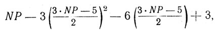
I. P lies on the curve… NP =3 • ON2 - 6 • ON + 3 . . .
II. P lies on the st. line, …2 • ON =• 3 • NP - 5 ... Thus x = ON, y = NP satisfy both the equations у - 3x2 - 6x + 3 and 2x = 3y - 5. It may similarly be shown that x = OM, y = MQ satisfy these equations. This is the first result given above.
| Also from II NP= | 2 . ON+ 5 | . |
| 3 |
Substituting this value of NP in I we have
| 2 .ON + 5 | =3 .ON2 - 6 .ON + 3, |
| 3 |
i, e. x = ONsatisfies the equation.
III.
| 2 x + 5 | =3x2 - 6x + 3... |
| М156 (03)89 |
It may similarly be shown that x = OM satisfies III.
But III is the equation obtained by eliminating У from the given equations. This is the second result given above.
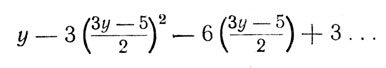
Again, from II
| ON = | 3 . NP - 5 | . |
| 2 |
Substituting this value of ON in I we have
i. e. у = NP satisfies the equation.
IV.
It may similarly be shown that у = Q satisfies IV.
But IV is the equation obtained by eliminating X from the given equations. third
This is the result given above.
It is easily seen that:
1) The solutions of the given simultaneous equations are x = 2, у = 3 and x = 0.2 approx.; y = 1.8 approx.
2) The solutions of the equation III are x = 2 and x = 0.2 approx.
3) The solutions of the equation IV are y = 3 and у = 1.8 approx.
The values 2,3 of X, У respectively are exact, as may easily be verified by substitution in the equations.
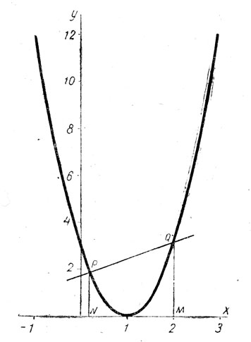
График параболы
The values 0.2, 1.8 are approximate only; if greater accuracy is required, we may draw a portion of the graphs on a very large scale in the neighbourhood of P. Since X is greater than 0.2, a suitable enlargement is the portion of the graphs between X = 0.21 and X = 0.24.
The values of X and Y are approximately 0.222 and 1.81 respectively.
The values obtained by calculation are
| x = | 2 | = 0,2 |
| 9 |
and
| y = 1 | 22 | = 1.814. |
| 27 |
Any degree of accuracy desired may be obtained by repeating the above process.
Note 1. In solving equations by drawing two graphs, it is essential that the scales for X shall be the same for each graph. But it is not necessary that the scale for X should be the same as the scale for Y.
Note 2. When we speak of graphs, it is implied that the same axes are used, and also that the same scales have been used for X for each graph, and also for Y.
One important result which follows from the general theorem is that graphical solutions of any quadratic equation may be obtained by drawing the graph of y = x2 and the graph of a straight line.
approx. = approximately приблизительно
binomial двучлен
dependent variable зависимая переменная
grasp the meaning of уловить (понять) смысл
independent независимый
index показатель
literal coefficient буквенный коэффициент
say зд. скажем
simultaneous equations система уравнений
squared paper миллиметровка
|
ПОИСК:
|
При использовании материалов сайта активная ссылка обязательна:
http://genling.ru/ 'Общее языкознание'